 MENU
MENU


NOTE!
Click on MENU to Browse between Subjects...17CS52 - COMPUTER NETWORKS
Answer Script for Module 3
Solved Previous Year Question Paper
CBCS SCHEME
COMPUTER NETWORKS
[As per Choice Based Credit System (CBCS) scheme]
(Effective from the academic year 2019 -2020)
SEMESTER - V
Subject Code 17CS52
IA Marks 40
Number of Lecture Hours/Week 04
Exam Marks 60
These Questions are being framed for helping the students in the "FINAL Exams" Only
(Remember for Internals the Question Paper is set by your respective teachers).
Questions may be repeated, just to show students how VTU can frame Questions.
- ADMIN
Dijkstra's algorithm computes the least-cost path from one node to all other nodes in the network.
Let us define the following notation:
i. u: source-node
ii. D(v): cost of the least-cost path from the source u to destination v.
iii. p(v): previous node (neighbor of v) along the current least-cost path from the source to v.
iv. N': subset of nodes; v is in N' if the least-cost path from the source to v is known.
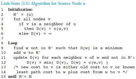
Fig 1.1: Link State Algorithm
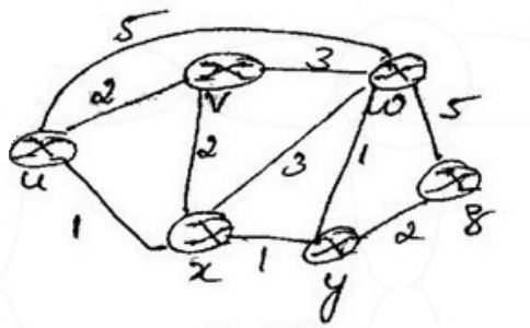
Example: Consider the network in Figure 1.2 and compute the least-cost paths from u to all possible destinations.
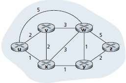
Fig 1.2: Abstract graph model of a computer network
Solution:
Let's consider the few first steps in detail.
i. In the initialization step, the currently known least-cost paths from u to its directly attached neighbors, v, x, and w, are initialized to 2, 1, and 5, respectively.
ii. In the first iteration, we
a. look among those nodes not yet added to the set N' and
b. find that node with the least cost as of the end of the previous iteration.
iii. In the second iteration,
a. nodes v and y are found to have the least-cost paths (2) and
b. we break the tie arbitrarily and
c. add y to the set N' so that N' now contains u, x, and y.
iv. And so on. . . .
v. When the LS algorithm terminates,
We have, for each node, its predecessor along the least-cost path from the source.
A tabular summary of the algorithm's computation is shown in Table 1.3.
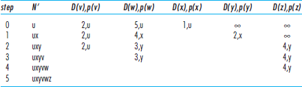
Fig 1.3: Running the link-state algorithm on the network in Figure 1.2
Figure 1.4 shows the resulting least-cost paths for u for the network in Figure 1.2.
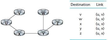
Fig 1.4: Least cost path and forwarding-table for node u
Routing.
The network layer must determine the route or path taken by packets as they
flow from a sender to a receiver. The algorithms that calculate these paths
are referred to as routing algorithms. A routing algorithm would determine,
for example, the path along which packets flow from H1 to H2.
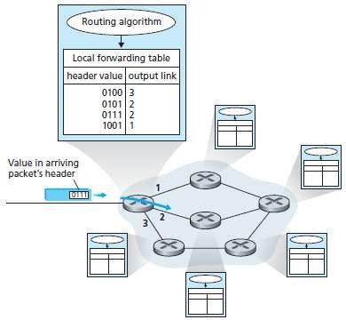
Fig 2.1: Routing algorithms determine values in forwarding tables.
As shown in Figure 2.1, the routing algorithm determines the values that are inserted into the routers' forwarding tables. The routing algorithm may be centralized (e.g., with an algorithm executing on a central site and downloading routing information to each of the routers) or decentralized (i.e., with a piece of the distributed routing algorithm running in each router). In either case, a router receives routing protocol messages, which are used to configure its forwarding table. The distinct and different purposes of the forwarding and routing functions can be further illustrated by considering the hypothetical (and unrealistic, but technically feasible) case of a network in which all forwarding tables are configured directly by human network operators physically present at the routers.
· The format of the IPv6 datagram is shown in Figure 3.1.
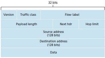
Fig 3.1: IPv6 datagram format
The following fields are defined in IPv6:
i. Version
a. This field specifies the IP version, i.e., 6.
ii. Traffic Class
a. This field is similar to the TOS field in IPv4.
b. This field indicates the priority of the packet.
iii. Flow Label
a. This field is used to provide special handling for a particular flow of data.
iv. Payload Length
a. This field shows the length of the IPv6 payload.
v. Next Header
a. This field is similar to the options field in IPv4 (Figure 3.19).
b. This field identifies type of extension header that follows the basic header.
vi. Hop Limit
a. This field is similar to TTL field in IPv4.
b. This field shows the maximum number of routers the packet can travel.
c. The contents of this field are decremented by 1 by each router that forwards the datagram.
d. If the hop limit count reaches 0, the datagram is discarded.
vii. Source & Destination Addresses
a. These fields show the addresses of the source & destination of the packet.
viii. Data
This field is the payload portion of the datagram.
When the datagram reaches the destination, the payload will be
a. removed from the IP datagram and
b. passed on to the upper layer protocol (TCP or UDP).
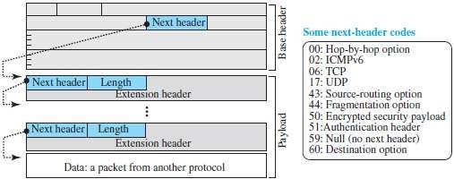
Fig 3.2: Payload in IPv6 datagram
· BGP is widely used for inter-AS routing in the Internet.
Using BGP, each AS cani. Obtain subnet reachability-information from neighboring ASs.
ii. Propagate the reachability-information to all routers internal to the AS.
iii. Determine good routes to subnets based on i) reachability-information and ii) AS policy.
· Using BGP, each subnet can advertise its existence to the rest of the Internet.
· Pairs of routers exchange routing-information over semi-permanent TCP connections using port-179.
· One TCP connection is used to connect 2 routers in 2 different autonomous-systems. Semi-permanent TCP connection is used to connect among routers within an autonomous-system.
· Two routers at the end of each connection are called peers.
The messages sent over the connection is called a session.
Two types of session:i. External BGP (eBGP) session
a. This refers to a session that spans 2 autonomous-systems.
ii. Internal BGP (iBGP) session
a. This refers to a session between routers in the same AS
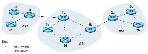
Fig 4.1: eBGP and iBGP sessions
· The destinations are not hosts but instead are CIDRized prefixes.
· Each prefix represents a subnet or a collection of subnets.
4.2 Path Attributes & Routes
· An autonomous-system is identified by its globally unique ASN (Autonomous-System Number).
· The router includes a number of attributes with the prefix.
· Two important attributes: 1) AS-PATH and 2) NEXT-HOP
i. AS-PATH
a. This attribute contains the ASs through which the advertisement for the prefix has passed.
b. When a prefix is passed into an AS, the AS adds its ASN to the ASPATH attribute.
c. Routers use the AS-PATH attribute to detect and prevent looping advertisements.
d. Routers also use the AS-PATH attribute in choosing among multiple paths to the same prefix.
ii. NEXT-HOP
e. This attribute provides the critical link between the inter-AS and intra-AS routing protocols.
f. This attribute is the router-interface that begins the AS-PATH.
BGP also includesa. attributes which allow routers to assign preference-metrics to the routes.
b. attributes which indicate how the prefix was inserted into BGP at the origin AS.
· When a gateway-router receives a route-advertisement, the gateway-router decides
a. whether to accept or filter the route and
b. whether to set certain attributes such as the router preference metrics.
1.3 Route Selection
· For 2 or more routes to the same prefix, the following elimination-rules are invoked sequentially:
i. Routes are assigned a local preference value as one of their attributes.
ii. The local preference of a route
a. will be set by the router or
b. will be learned by another router in the same AS.
iii. From the remaining routes, the route with the shortest AS-PATH is selected.
iv. From the remaining routes, the route with the closest NEXT-HOP router is selected.
v. If more than one route still remains, the router uses BGP identifiers to select the route.
1.4 Routing Policy
· Routing policy is illustrated as shown in Figure 3.30.
· Let A, B, C, W, X & Y = six interconnected autonomous-systems. W, X & Y = three stub-networks.
a. A, B & C = three backbone provider networks.
All traffic entering a stub-network must be destined for that network.a. All traffic leaving a stub-network must have originated in that network.
· X is a multi-homed stub-network, since X is connected to the rest of the n/w via 2 different providers
· X itself must be the source/destination of all traffic leaving/entering X.
· X will function as a stub-network if X has no paths to other destinations except itself.
· There are currently no official standards that govern how backbone ISPs route among themselves.
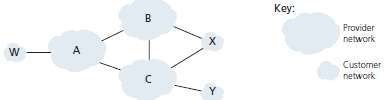
Fig 4.2: A simple BGP scenario
5.1
Broadcast Routing Algorithms
Broadcast-routing means delivering a packet from a source-node to all other nodes in the network
5.2
Some of the Broadcast Routing Algorithms
a. Center Based Approach
5.3 N-way Unicast
a. makes N copies of the packet and
b. transmits then the N copies to the N destinations using unicast routing (Figure 5.1).
i. Inefficiency
If source is connected to the n/w via single link, then N copies of packet will traverse this link.
ii. More Overhead & Complexity
An implicit assumption is that the sender knows broadcast recipients and their addresses.
Obtaining this information adds more overhead and additional complexity to a protocol.
iii. Not suitable for Unicast Routing
It is not good idea to depend on the unicast routing infrastructure to achieve broadcast.
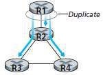
Fig 5.1: Duplicate creation/transmission
5.4 Uncontrolled Flooding
· The source-node sends a copy of the packet to all the neighbors.
· When a node receives a broadcast-packet, the node duplicates & forwards packet to all neighbors.
· In connected-graph, a copy of the broadcast-packet is delivered to all nodes in the graph.
i. If the graph has cycles, then copies of each broadcast-packet will cycle indefinitely.
ii. When a node is connected to 2 other nodes, the node creates & forwards multiple copies of packet
The endless multiplication of broadcast-packets which will eventually make the network useless."
5.5 Controlled Flooding
· A node can avoid a broadcast-storm by judiciously choosing
· when to flood a packet and when not to flood a packet.
i. Sequence Number Controlled Flooding
A source-node: puts its address as well as a broadcast sequence-number into a broadcast-packet.
a. Each node maintains a list of the source-address & sequence # of each broadcast-packet.
b. When a node receives a broadcast-packet, the node checks whether the packet is in this list.
c. If so, the packet is dropped; if not, the packet is duplicated and forwarded to all neighbors.
ii. Reverse Path Forwarding (RPF)
a. If a packet arrived on the link that has a path back to the source; Then the router transmits the packet on all outgoing-links. Otherwise, the router discards the incoming-packet.
b.Such a packet will be dropped. This is because the router has already received a copy of this packet (Figure 5.2).
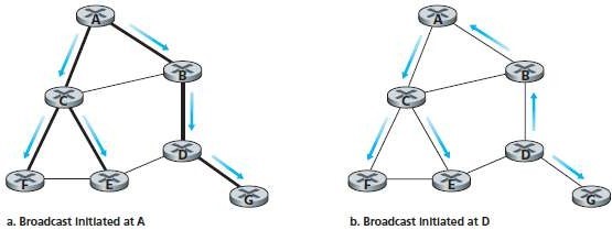
Fig 5.2: Reverse path forwarding
5.6 Spanning - Tree Broadcast
· This is another approach to providing broadcast. (MST Minimum Spanning Tree).
· Spanning-tree is a tree that contains each and every node in a graph.
· A spanning-tree whose cost is the minimum of all of the graph's spanning-trees is called a MST.
i. Firstly, the nodes construct a spanning-tree.
ii. The node sends broadcast-packet out on all incident links that belong to the spanning-tree.
iii. The receiving-node forwards the broadcast-packet to all neighbors in the spanning-tree.
Fig 5.3: Broadcast along a spanning-tree
Complex: The main complexity is the creation and maintenance of the spanning-tree.
5.6.1 Center Based Approach
i. A center-node (rendezvous point or a core) is defined.
ii. Then, the nodes send unicast tree-join messages to the center-node.
iii. Finally, a tree-join message is forwarded toward the center until the message either
a. arrives at a node that already belongs to the spanning-tree
b. (or)
c. arrives at the center.
· Figure 5.4 illustrates the construction of a center-based spanning-tree.
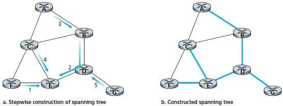
Fig 5.4: Center-based construction of a spanning-tree
Below Page NAVIGATION Links are Provided...
All the Questions on Question Bank Is SOLVED
Follow our Instagram Page:
FutureVisionBIE
https://www.instagram.com/futurevisionbie/
Message: I'm Unable to Reply to all your Emails
so, You can DM me on the Instagram Page & any other Queries.