Answer:

1.1 Disk Scheduling Algorithm (Introduction):

One of the responsibilities of the operating system is to use the hardware efficiently. For the disk drives, meeting this responsibility entails having fast access time and large disk bandwidth.

The access time has two major components.

The seek time

is the time for the disk arm to move the heads to the cylinder containing the desired sector.

The rotational latency

is the additional time for the disk to rotate the desired sector to the disk head.

The

disk bandwidth

is the total number of bytes transferred, divided by the total time between the first request for service and the completion of the last transfer. We can improve both the access time and the bandwidth by scheduling the servicing of disk I/O requests in a good order

Whenever a process needs I/O to or from the disk, it issues a system call to the operating system. The request specifies several pieces of information:

i. Whether this operation is input or output

ii. What the disk address for the transfer is

iii. What the memory address for the transfer is

iv. What the number of sectors to be transferred is

If the desired disk drive and controller are available, the request can be serviced immediately. If the drive or controller is busy, any new requests for service will be placed in the queue of pending requests for that drive.

The various Disk Scheduling algorithms are as follows:

i. FCFS Scheduling

ii. SSTF Scheduling

iii. SCAN Scheduling

iv. C-SCAN Scheduling

v. LOOK Scheduling

vi. Selection of a Disk-Scheduling Algorithm

1.2 FCFS Scheduling:

The simplest form of disk scheduling is, of course, the first-come, first-served (FCFS) algorithm. This algorithm is intrinsically fair, but it generally does not provide the fastest service. Consider, for example, a disk queue with requests for I/O to blocks on cylinders

98, 183, 37,122, 14, 124, 65, 67

in that order. If the disk head is initially at cylinder 53, it will first move from 53 to 98, then to 183, 37, 122, 14, 124/65, and finally to 67, for a total head movement of 640 cylinders. This schedule is diagrammed in Figure 1.1.

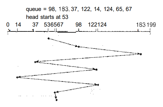
Fig 1.1 FCFS disk scheduling

The wild swing from 122 to 14 and then back to 124 illustrates the problem with this schedule. If the requests for cylinders 37 and 14 could be serviced together, before or after the requests at 122 and 124, the total head movement could be decreased substantially, and performance could be thereby improved.

1.3 SSTF Scheduling

It seems reasonable to service all the requests close to the current head position before moving the head far away to service other requests. This assumption is the basis for the

shortest-seek-time-first (SSTF) algorithm

.

The

SSTF algorithm

selects the request with the minimum seek time from the current head position. Since seek time increases with the number of cylinders traversed by the head, SSTF chooses the pending request closest to the current head position.

For our

example

request queue, the closest request to the initial head position (53) is at cylinder 65. Once we are at cylinder 65, the next closest request is at cylinder 67. From there, the request at cylinder 37 is closer than the one at 98, so 37 is served next. Continuing, we service the request at cylinder 14, then 98,122, 124, and finally 183 (Figure 1.2).

This

scheduling

method results in a total head movement of only 236 cylinders-little more than one-third of the distance needed for FCFS scheduling of this request queue. This algorithm gives a

substantial improvement in performance

.

SSTF scheduling

is essentially a form of

shortest-job-first (SJF) scheduling

; and like SJF scheduling, it may cause starvation of some requests. Remember that requests may arrive at any time. Suppose that we have two requests in the queue, for cylinders 14 and 186, and while servicing the request from 14, a new request near 14 arrives.

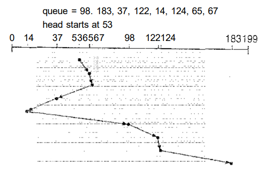
Fig 1.2 SSTF disk scheduling.

This new request will be serviced next, making the request at 186 wait. While this request is being serviced, another request close to 14 could arrive. In theory, a continual stream of requests near one another could arrive, causing the request for cylinder 186 to wait indefinitely. This scenario becomes increasingly likely if the pending-request queue grows long.

1.4 SCAN Scheduling:

In the

SCAN algorithm

, the disk arm starts at one end of the disk and moves toward the other end, servicing requests as it reaches each cylinder, until it gets to the other end of the disk. At the other end, the direction of head movement is reversed, and servicing continues. The head continuously scans back and forth across the disk.

The

SCAN algorithm

is sometimes called the elevator algorithm, since the disk arm behaves just like an elevator in a building, first servicing all the requests going up and then reversing to service requests the other way.

Let's return to our

example

to illustrate. Before

applying SCAN

to schedule the requests on cylinders

98,183, 37,122,14, 124, 65, and 67

, we need to know the direction of head movement in addition to the head's current position (53). If the disk arm is moving toward 0, the head will service 37 and then 14. At cylinder 0, the arm will reverse and will move toward the other end of the disk, servicing the requests at 65, 67, 98, 122, 124, and 183 (Figure 1.3).

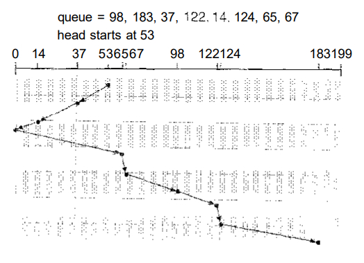
Fig 1.3 SCAN disk scheduling

If a request arrives in the queue just in front of the head, it will be serviced almost immediately; a request arriving just behind the head will have to wait until the arm moves to the end of the disk, reverses direction, and comes back.

Assuming a

uniform distribution of requests

for cylinders, consider the density of requests when the head reaches one end and reverses direction. At this point, relatively few requests are immediately in front of the head, since these cylinders have recently been serviced. The heaviest density of requests is at the other end of the disk

1.5 C-SCAN Scheduling:

Circular SCAN (C-SCAN) scheduling

is a variant of SCAN designed to provide a more uniform wait time.

Like SCAN, C-SCAN

moves the head from one end of the disk to the other, servicing requests along the way. When the head reaches the other end, however, it immediately returns to the beginning of the disk, without servicing any requests on the return trip (Figure 1.4).

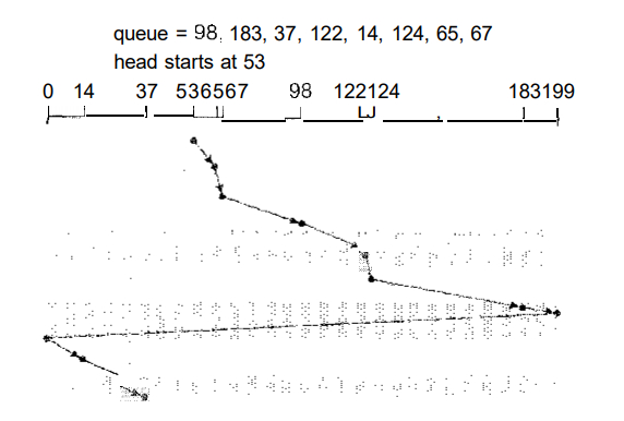
Fig 1.4 C-SCAN disk scheduling.

The

C-SCAN scheduling algorithm

essentially treats the cylinders as a circular list that wraps around from the final cylinder to the first one.

1.6 LOOK Scheduling:

As we described them, both

SCAN and C-SCAK

move the disk arm across the full width of the disk. In practice, neither algorithm is often implemented this way. More commonly, the arm goes only as far as the final request in each direction.

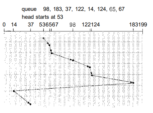
Fig 1.5 C-LOOK disk scheduling.

Then, it reverses direction immediately, without going all the way to the end of the disk. Versions of

SCAN and C-SCAN

that follow this pattern are called

LOOK and C-LOOK scheduling

, because they look for a request before continuing to move in a given direction (Figure 1.5).

1.7 Selection of a Disk-Scheduling Algorithm:

SSTF is commonly used and it increases performance over FCFS. SCAN and C-SCAN algorithm is better for a heavy load on disk. SCAN and C-SCAN have less starvation problem.

Disk scheduling algorithm should be written as a separate module of the operating system. SSTF or Look is a reasonable choice for a default algorithm.

SSTF is commonly used algorithms has it has a less seek time when compared with other algorithms. SCAN and C-SCAN perform better for systems with a heavy load on the disk, (ie. more read and write operations from disk).

Selection of disk scheduling algorithm is influenced by the file allocation method, if contiguous file allocation is chosen, then FCFS is best suitable, because the files are stored in contiguous blacks and there will be limited head movements required. A linked or indexed file, in contrast, may include blocks that are widely scattered on the disk, resulting in greater head movement.

The location of directories and index blocks is also important. Since every file must be opened to be used, and opening a file requires searching the directory structure, the directories will be accessed frequently. Suppose that a directory entry is on the first cylinder and a file's data are on the final cylinder. The disk head has to move the entire width of the disk. If the directory entry were on the middle cylinder, the head would have to move, at most, one-half the width. Caching the directories and index blocks in main memory can also help to reduce the disk-arm movement, particularly for read requests.

Because of these complexities, the disk-scheduling algorithm is very important and is written as a separate module of the operating system.

Answer:

Our model of protection can be viewed abstractly as a matrix, called an access matrix. The rows of the access matrix represent domains, and the columns represent objects. Each entry in the matrix consists of a set of access rights. Because the column defines objects explicitly, we can omit the object name from the access right. The entry access (i, j) defines the set of operations that a process executing in domain D1 can invoke on object Oj.

To illustrate these concepts, we consider the access matrix shown in Figure 2.1. There are four domains and four objects-three files (F1, F2, F3) and one laser printer. A process executing in domain D1 can read files F1 and F3. A process executing in domain D4 has the same privileges as one executing in domain D1; but in addition, it can also write onto files F1 and F3. Note that the laser printer can be accessed only by a process executing in domain D0

Fig 1.1 Access Matrix

The access-matrix scheme provides us with the mechanism for specifying a variety of policies. The mechanism consists of implementing the access matrix and ensuring that the semantic properties we have outlined indeed, hold. More specifically, we must ensure that a process executing in domain D1, can access only those objects specified in row 1, and then only as allowed by the access-matrix entries.

The access matrix can implement policy decisions concerning protection. The policy decisions involve which rights should be included in the (i. j)th entry. We must also decide the domain in which each process executes. This last policy is usually decided by the operating system.

The users normally decide the contents of the access-matrix entries. When a user creates a new object Oi, the column Oj is added to the access matrix with the appropriate initialization entries, as dictated by the creator. The user may decide to enter some rights in some entries in column 1 and other rights in other entries, as needed.

The access matrix provides an appropriate mechanism for defining and implementing strict control for both the static and dynamic association between processes and domains. When we switch a process from one domain to another, we are executing an operation (switch) on an object (the domain). We can control domain switching by including domains among the objects of the access matrix.

Similarly, when we change the content of the access matrix, we are performing an operation on an object: the access matrix. Again, we can control these changes by including the access matrix itself as an object. Actually, since each entry in the access matrix may be modified individually, we must consider each entry in the access matrix as an object to be protected. Now, we need to consider only the operations possible on these new objects (domains and the access matrix) and decide how we want processes to be able to execute these operations.

Processes should be able to switch from one domain to another. Domain switching from domain Di to domain Dj is allowed if and only if the access right switch access(I, j). Thus, in Figure 2.2, a process executing in domain D2 can switch to domain D3 or to domain D4. A process in domain D4 can switch to D1, and one in domain D1 can switch to domain D2.

(b)

Fig 2.3 Access matrix with copy rights

The ability to copy an access right from one domain (or row) of the access matrix to another is denoted by an asterisk (*) appended to the access right. The copy right allows the copying of the access right only within the column (that is, for the object) for which the right is defined. For example, in Figure 2.3(a), a process executing in domain D2 can copy the read operation into any entry associated with file F2. Hence, the access matrix of Figure 2.3(a) can be modified to the access matrix shown in Figure 2.3(b).

This scheme has two variants:

i. A right is copied from access (i, l) to access(k, j); it is then removed from access (i, j). This action is a transfer of a right, rather than a copy.

ii. Propagation of the copy right may be limited. That is, when the right R* is copied from access (I, j) to access (k, j), only the right R (not R*) is created. A process executing in domain D_k cannot further copy the right R.

A system may select only one of these three copy rights, or it may provide all three by identifying them as separate rights: copy, transfer, and limited copy.

Answer:

3.1 Components of a Linux System:

The Linux system is composed of three main bodies of code, in line with most traditional UNIX implementations:

1. Kernel.

The kernel is responsible for maintaining all the important abstractions of the operating system, including such things as virtual memory and processes.

2. System libraries.

The system libraries define a standard set of functions through which applications can interact with the kernel. These functions implement much of the operating-system functionality that does not need the full privileges of kernel code.

3. System utilities.

The system utilities are programs that perform individual, specialized management tasks. Some system utilities may be invoked just once to initialize and configure some aspect of the system; others- known as daemons in UNIX terminology-may run permanently, handling such tasks as responding to incoming network connections, accepting logon requests from terminals, and updating log files.

Figure 3.1 illustrates the various components that make up a full Linux system. The most important distinction here is between the kernel and everything else.

All the kernel code executes in the processor's privileged mode with full access to all the physical resources of the computer. Linux refers to this privileged mode as

kernel mode

.

Fig 3.1 Components of the Linux system.

Under Linux, no user-mode code is built into the kernel. Any operating-system-support code that does not need to run in kernel mode is placed into the system libraries instead.

Although various modern operating systems have adopted a message passing architecture for their kernel internals, Linux retains UNIX's historical model: The kernel is created as a single, monolithic binary.

The

main reason

is to improve performance: Because all kernel code and data structures are kept in a single address space, no context switches are necessary when a process calls an operating-system function or when a hardware interrupt is delivered.

Not only

the core scheduling and virtual memory code

occupies this address space; all kernel code, including all device drivers, file systems, and networking code, is present in the same single address space.

The

Linux kernel

forms the core of the Linux operating system. It provides all the functionality necessary to run processes, and it provides system services to give arbitrated and protected access to hardware resources.

The

kernel implements

all the features required to qualify as an operating system. On its own, however, the operating system provided by the Linux kernel looks nothing like a UNIX system.

The

operating-system interface

visible to running applications is not maintained directly by the kernel. Rather, applications make calls to the system libraries, which in turn call the operating system services as necessary.

The system libraries

provide many types of functionality. At the simplest level, they allow applications to make kernel-system-service requests. Making a system call involves transferring control from unprivileged user mode to privileged kernel mode; the details of this transfer vary from architecture to architecture.

The

libraries

take care of collecting the system-call arguments and, if necessary, arranging those arguments in the special form necessary to make the system call.

The libraries may also provide more complex versions of the basic system calls.

For example

, the C language's buffered file-handling functions are all implemented in the system libraries, providing more advanced control of file I/O than the basic kernel system calls.

Answer:

4.1 Inter Process communication - IPC:

UNIX provides a rich environment for processes to communicate with each other. Communication may be just a matter of letting another process know that some event has occurred, or it may involve transferring data from one process to another.

4.2 Synchronization and Signals:

The standard UNIX

mechanism

for informing a process that an event has occurred is the signal. Signals can be sent from any process to any other process, with restrictions on signals sent to processes owned by another user. However, a limited number of signals are available, and they cannot carry information: Only the fact that a signal occurred is available to a process. Signals are not generated only by processes.

The

kernel

also generates signals internally; for example, it can send a signal to a server process when data arrive on a network channel, to a parent process when a child terminates, or to a waiting process when a timer expires.

Internally, the

Linux kernel

does not use signals to communicate with processes running in kernel mode. If a

kernel-mode process

is expecting an event to occur, it will not normally use signals to receive notification of that event. Rather,

communication

about incoming asynchronous events within the kernel is performed through the use of scheduling states and wait queue structures.

These

mechanisms

allow

kernel-mode processes

to inform one another about relevant events, and they also allow events to be generated by device drivers or by the networking system. Whenever a process wants to wait for some event to complete, it places itself on a

wait queue

associated with that event and tells the scheduler that it is no longer eligible for execution.

Once the event

has completed

, it will wake up every process on the wait queue. This procedure allows multiple processes to wait for a single event. For example, if several processes are trying to

read a file from a disk

, then they will all be awakened once the data have been read into memory successfully.

4.3 Passing of Data Among Processes:

Linux offers several

mechanisms for passing data among processes

. The standard UNIX pipe mechanism allows a child process to inherit a communication channel from its parent; data written to one end of the pipe can be read at the other.

Under

Linux, pipes

appear as just another type of inode to virtual-file system software, and each pipe has a pair of wait queues to

synchronize

the reader and writer. UNIX also

defines

a set of networking facilities

that can send streams of data to both local and remote processes.

Two other methods of sharing data among processes are available.

First, shared memory

offers an extremely fast way to communicate large or small amounts of data; any data written by one process to a

shared memory region

can be read immediately by any other process that has mapped that region into its address space.

The main

disadvantage of shared memory

is that, on its own, it offers no synchronization: A process can neither ask the operating system whether a piece of shared memory has been written to nor suspend execution until such a write occurs.

Shared memory becomes particularly powerful when used in conjunction with another

inter-process-communication mechanism

that provides the missing synchronization.

A

shared-memory region in Linux

is a persistent object that can be created or deleted by processes. Such an object is treated as though it were a small independent address space.

The

Linux paging algorithms

can elect to page out to disk shared-memory pages, just as they can page out a process's data pages. The shared-memory object acts as a backing store for shared-memory regions, just as a file can act as a backing store for a memory-mapped memory region.

When a

file is mapped

into a

virtual-address-space region

, then any page faults that occur cause the appropriate page of the file to be mapped into virtual memory.

Similarly,

shared-memory mappings direct page faults

to map in pages from a persistent shared-memory object. Also just as for files, shared memory objects remember their contents even if no processes are currently mapping them into virtual memory.

Answer:

Linux has

two separate process-scheduling algorithms

.

One is a

time-sharing algorithm

for fair, premptive scheduling among multiple processes.

the other is designed for

real-time tasks

, where absolute priorities are more important than fairness.

The scheduling algorithm used for routine, time-sharing tasks received a major overhaul with version 2.5 of the kernel. Prior to version 2.5, the Linux kernel ran a variation of the traditional

UNIX scheduling algorithm

.

Among other issues, problems with the traditional UNIX scheduler are that it does not provide adequate support for SMP systems and that it does not scale well as the number of tasks on the system grows.

The

overhaul

of the scheduler

with version 2.5 of the kernel now provides a scheduling algorithm that runs in constant time-known

as O(l)

regardless of the number of tasks on the system. The new scheduler also provides increased support for

SMP

, including processor affinity and load balancing, as well as maintaining fairness and support for interactive tasks.

The

Linux scheduler

is a pre-emptive, priority-based algorithm with two separate priority ranges: a real-time range from 0 to 99 and a nice value ranging from 100 to 140. These two ranges map into a global priority scheme whereby numerically lower values indicate higher priorities.

Unlike

schedulers f

or many other systems, Linux assigns higher-priority tasks longer time quanta and vice-versa. Because of the unique nature of the scheduler, this is appropriate for Linux, as we shall soon see. The relationship between priorities and time-slice length is shown in Figure 5.1.

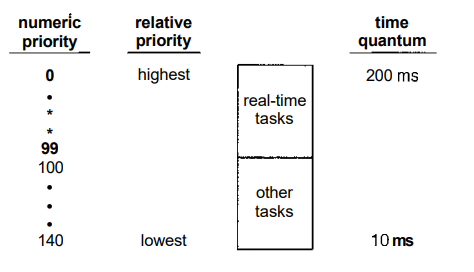
Fig 5.1 The relationship between priorities and time-slice length.

A

runnable task is considered

eligible for execution on the

CPU

so long as it has time remaining in its time slice. When a task has exhausted its time slice, it is considered

expired

and is not eligible for execution again until all other tasks have also exhausted their time quanta.

The kernel maintains a list of all

runnable

tasks in a run queue data structure. Because of its support for SMP, each processor maintains its own run queue and schedules itself independently. Each run queue contains two priority arrays

active and expired

.

The

active array

contains all tasks with time remaining in their time slices, and the expired array contains all expired tasks. Each of these priority arrays includes a list of tasks indexed according to priority (Figure 5.2).

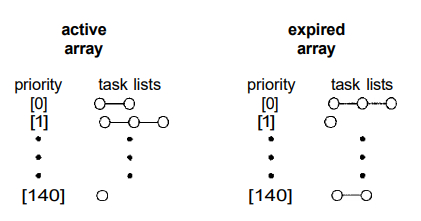
Fig 5.2 List of tasks indexed according to priority.

The

scheduler chooses

the task with the highest priority from the active array for execution on the CPU. On multiprocessor machines, this means that each processor is scheduling the highest-priority task from its own run queue structure.

When all tasks have

exhausted their time slices

(that is, the active array is empty), the two priority arrays are exchanged as the expired array becomes the active array and vice-versa